Trend Channel SwiftEdgeTrend Channel SwiftEdge
The Trend Channel SwiftEdge is a powerful, visually striking tool designed to help traders identify trends and potential trade setups across multiple timeframes with a futuristic, tech-inspired design. This indicator combines a dynamic trend channel with a multi-timeframe trend dashboard and intelligent signal filtering to provide clear, actionable insights for both novice and experienced traders. Its unique neon-lit, holographic visuals give it a modern, cutting-edge feel, making your chart analysis both functional and visually engaging.
What It Does
This indicator identifies trends on your chart using a dynamic price channel and provides buy and sell signals based on trend alignments across multiple timeframes. It also features a dashboard that displays the trend direction (Up, Down, or Neutral) for six timeframes: 1-minute, 5-minute, 15-minute, 1-hour, 4-hour, and 1-day. The signals are filtered using a user-selected higher timeframe to ensure they align with broader market trends, reducing noise and improving trade reliability.
How It Works
The Trend Channel SwiftEdge operates in three key steps:
Dynamic Trend Channel:
A moving average (MA) is calculated based on your chosen type (SMA, EMA, or WMA) and length (default is 14 periods). This MA forms the backbone of the trend channel.
The channel’s upper and lower bounds are created by calculating the highest and lowest values of the MA over a period (default is 2x the MA length). These bounds help identify the trend: if the price is above the upper channel, the trend is Up; if below the lower channel, the trend is Down; otherwise, it’s Neutral.
The MA and channel lines are plotted with neon colors (green for Up, red for Down, blue for the channel bounds) to create a holographic effect, with a glowing background fill between the channels to highlight the trend direction.
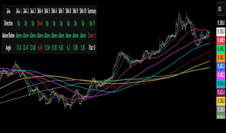
Multi-Timeframe Trend Dashboard:
The indicator analyzes trends across six timeframes (1M, 5M, 15M, 1H, 4H, D1) using the same trend channel logic.
A dashboard in the top-right corner displays each timeframe’s trend direction with a futuristic design: neon green for Up, neon red for Down, and gray for Neutral, all set against a dark background with neon blue accents.
Signal Generation with Higher Timeframe Filter:
Buy and Sell signals are generated when the trend on the chart’s timeframe (e.g., 1M) aligns with a user-selected higher timeframe (e.g., 15M).
A Buy signal ("🚀 SwiftEdge BUY") appears when the price crosses above the upper channel (indicating an Up trend) and the selected higher timeframe’s trend also turns Up. If the higher timeframe is Neutral, the indicator checks even higher timeframes (e.g., 1H and 4H for a 15M filter) to confirm the trend direction.
A Sell signal ("🛑 SwiftEdge SELL") appears when the price crosses below the lower channel (indicating a Down trend) and the selected higher timeframe’s trend turns Down, with the same higher timeframe check for Neutral cases.
Signals are displayed as neon-colored labels with emojis for a futuristic touch, making them easy to spot.
Why This Combination?
The combination of a dynamic trend channel, multi-timeframe analysis, and signal filtering in Trend Channel SwiftEdge is designed to provide a comprehensive view of market trends while reducing false signals. The trend channel identifies the primary trend on your chart, while the multi-timeframe dashboard ensures you’re aware of the broader market context. The signal filter leverages higher timeframes to confirm that your trades align with larger trends, which is particularly useful in volatile markets where smaller timeframes can be noisy. This synergy creates a balanced approach, blending short-term precision with long-term trend confirmation, all wrapped in a visually engaging tech-inspired design.
How to Use It
Add the Indicator: Apply Trend Channel SwiftEdge to your TradingView chart.
Customize Settings:
SwiftEdge Moving Average Type: Choose between SMA, EMA, or WMA (default is EMA) to adjust the trend channel’s sensitivity.
SwiftEdge MA Length: Set the period for the moving average (default is 14).
SwiftEdge Signal Filter Timeframe: Select a higher timeframe (1M, 5M, 15M, 1H, 4H, D1) to filter signals (default is 15M). For example, on a 1M chart, selecting 15M ensures signals align with the 15-minute trend.
Show SwiftEdge Ribbon: Toggle the visibility of the trend channel’s moving average (default is true).
Show SwiftEdge Background Glow: Toggle the glowing background fill between the channel bounds (default is true).
Start/End Year: Set a time range for the indicator’s signals (default is 1900–2100).
Interpret the Dashboard: Check the top-right dashboard to see the trend direction across all timeframes. Use this to understand the broader market context.
Trade with Signals:
Look for "🚀 SwiftEdge BUY" labels (neon green) below candles to enter long positions when the trend aligns across timeframes.
Look for "🛑 SwiftEdge SELL" labels (neon red) above candles to enter short positions or exit longs.
Ensure the signal aligns with your trading strategy and risk management.
What Makes It Original?
Trend Channel SwiftEdge stands out with its futuristic, tech-inspired design and multi-timeframe synergy. Unlike traditional trend indicators, it combines a visually striking neon aesthetic with practical functionality, making trend analysis both intuitive and engaging. The signal filtering mechanism, which checks higher timeframes dynamically, ensures trades are backed by broader market trends, reducing the risk of false signals. The dashboard provides a quick, at-a-glance view of trends across multiple timeframes, empowering traders to make informed decisions without needing to switch charts. This blend of advanced trend analysis, intelligent signal filtering, and a high-tech visual theme makes it a unique tool for modern traders.
Notes
Best used on trending markets; in choppy conditions, consider using higher timeframes for signal filtering to reduce noise.
Adjust the MA length and signal timeframe based on your trading style (shorter for scalping, longer for swing trading).
Why This Description Complies with TradingView House Rules
What It Does:
Clearly explains that the script identifies trends using a dynamic channel, provides buy/sell signals, and displays a multi-timeframe dashboard.
How It Does It:
Breaks down the process into three steps: trend channel calculation, multi-timeframe analysis, and signal generation with higher timeframe filtering.
Explains the logic (e.g., price crossing the channel, trend alignment across timeframes) in simple terms.
How to Use It:
Provides step-by-step instructions on adding the indicator, customizing settings, interpreting the dashboard, and trading with signals.
What Makes It Original:
Highlights the unique tech-inspired design, the combination of trend channel and multi-timeframe filtering, and the dynamic higher timeframe check.
Justifies the Combination:
Explains why the trend channel, multi-timeframe dashboard, and signal filtering are used together: to balance short-term precision with long-term trend confirmation, reducing false signals.
Self-Contained:
All concepts (trend channel, multi-timeframe analysis, signal filtering) are explained within the description without requiring external research.
Avoids technical jargon that would confuse non-Pine readers, focusing on user-friendly language.
This updated description with the new name "Trend Channel SwiftEdge" should fully comply with TradingView’s House Rules. If you need further adjustments, let me know!
Pine Script® göstergesi